TensorFlow GANs

Introduction

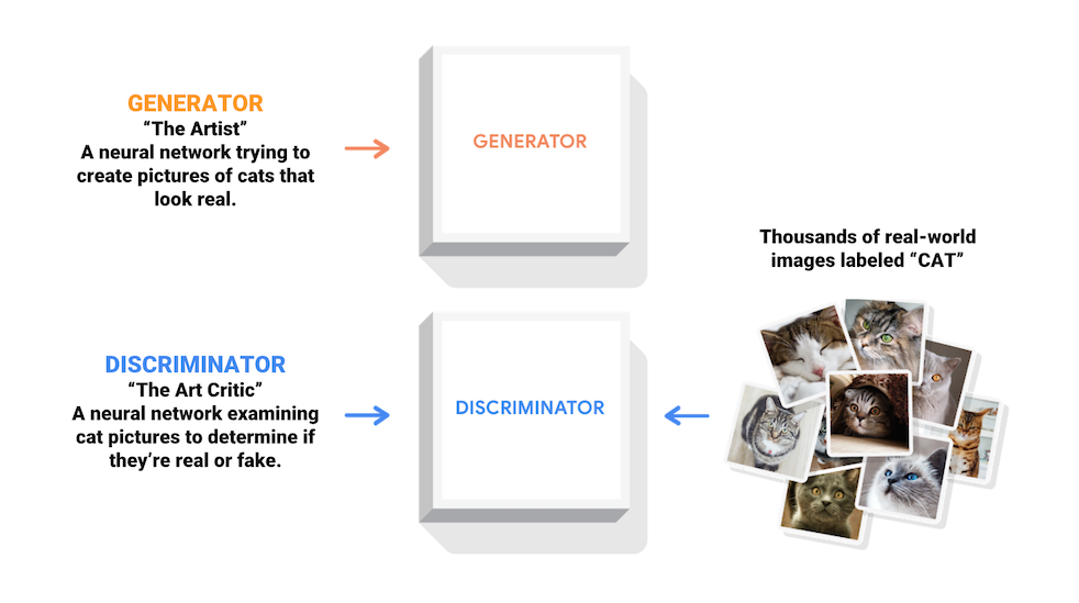
Generative Adversarial Networks (GANs) are one of the most fascinating developments in deep learning. Introduced by Ian Goodfellow and his colleagues in 2014, GANs consist of two neural networks—a Generator and a Discriminator—that compete against each other in a minimax game. The Generator tries to create data that looks real, while the Discriminator tries to distinguish between real and generated data. Through this adversarial process, the Generator improves at creating increasingly realistic data.

In this tutorial, we'll explore how to implement GANs using TensorFlow, Google's powerful deep learning framework. By the end, you'll understand the basic concepts behind GANs and be able to implement a simple GAN to generate images.

Understanding GANs

The GAN Architecture

A GAN consists of two main components:

1. Generator: Takes random noise as input and transforms it into data (like images)
2. Discriminator: Receives data (either real or generated) and outputs a probability indicating whether the input is real or fake

The training process involves:

• Training the Discriminator to correctly classify real and fake data
• Training the Generator to fool the Discriminator by creating realistic data

This adversarial setup creates a dynamic where both networks continuously improve, leading to more realistic generated data over time.

Implementing a Basic GAN with TensorFlow

Let's implement a simple GAN to generate handwritten digits similar to those in the MNIST dataset.

Setting Up the Environment

First, let's import the required libraries:

python

import tensorflow as tf
import numpy as np
import matplotlib.pyplot as plt
import time

from tensorflow.keras.layers import Dense, Flatten, Reshape, LeakyReLU, Dropout
from tensorflow.keras.models import Sequential
from tensorflow.keras.optimizers import Adam

Loading and Preparing the Data

We'll use the MNIST dataset of handwritten digits:

python

# Load MNIST dataset
(x_train, _), (_, _) = tf.keras.datasets.mnist.load_data()

# Normalize images to [-1, 1]
x_train = (x_train - 127.5) / 127.5
x_train = x_train.reshape(x_train.shape[0], 28, 28, 1).astype('float32')

# Batch and shuffle the data
BUFFER_SIZE = 60000
BATCH_SIZE = 256
train_dataset = tf.data.Dataset.from_tensor_slices(x_train).shuffle(BUFFER_SIZE).batch(BATCH_SIZE)

Building the Generator

The Generator transforms random noise into images:

python

def build_generator():
    model = Sequential([
        # Start with a Dense layer that takes in the noise
        Dense(7*7*256, use_bias=False, input_shape=(100,)),
        LeakyReLU(),
        Reshape((7, 7, 256)),
        
        # First transposed convolution layer
        tf.keras.layers.Conv2DTranspose(128, (5, 5), strides=(1, 1), padding='same', use_bias=False),
        tf.keras.layers.BatchNormalization(),
        LeakyReLU(),
        
        # Second transposed convolution layer
        tf.keras.layers.Conv2DTranspose(64, (5, 5), strides=(2, 2), padding='same', use_bias=False),
        tf.keras.layers.BatchNormalization(),
        LeakyReLU(),
        
        # Output layer with tanh activation
        tf.keras.layers.Conv2DTranspose(1, (5, 5), strides=(2, 2), padding='same', use_bias=False, activation='tanh')
    ])
    
    return model

Building the Discriminator

The Discriminator classifies images as real or fake:

python

def build_discriminator():
    model = Sequential([
        # First convolutional layer
        tf.keras.layers.Conv2D(64, (5, 5), strides=(2, 2), padding='same', input_shape=[28, 28, 1]),
        LeakyReLU(),
        Dropout(0.3),
        
        # Second convolutional layer
        tf.keras.layers.Conv2D(128, (5, 5), strides=(2, 2), padding='same'),
        LeakyReLU(),
        Dropout(0.3),
        
        # Output layer
        Flatten(),
        Dense(1)  # No activation (will use sigmoid in the loss function)
    ])
    
    return model

Defining Loss Functions and Optimizers

We'll use the binary cross-entropy loss and the Adam optimizer:

python

# Loss functions
cross_entropy = tf.keras.losses.BinaryCrossentropy(from_logits=True)

def discriminator_loss(real_output, fake_output):
    real_loss = cross_entropy(tf.ones_like(real_output), real_output)
    fake_loss = cross_entropy(tf.zeros_like(fake_output), fake_output)
    total_loss = real_loss + fake_loss
    return total_loss

def generator_loss(fake_output):
    return cross_entropy(tf.ones_like(fake_output), fake_output)

# Optimizers
generator_optimizer = tf.keras.optimizers.Adam(1e-4)
discriminator_optimizer = tf.keras.optimizers.Adam(1e-4)

Creating the Training Loop

Now, let's define the training step and the complete training loop:

python

@tf.function
def train_step(images):
    noise = tf.random.normal([BATCH_SIZE, 100])
    
    with tf.GradientTape() as gen_tape, tf.GradientTape() as disc_tape:
        # Generate fake images
        generated_images = generator(noise, training=True)
        
        # Get Discriminator outputs for real and fake images
        real_output = discriminator(images, training=True)
        fake_output = discriminator(generated_images, training=True)
        
        # Calculate losses
        gen_loss = generator_loss(fake_output)
        disc_loss = discriminator_loss(real_output, fake_output)
        
    # Calculate gradients
    gradients_of_generator = gen_tape.gradient(gen_loss, generator.trainable_variables)
    gradients_of_discriminator = disc_tape.gradient(disc_loss, discriminator.trainable_variables)
    
    # Apply gradients
    generator_optimizer.apply_gradients(zip(gradients_of_generator, generator.trainable_variables))
    discriminator_optimizer.apply_gradients(zip(gradients_of_discriminator, discriminator.trainable_variables))
    
    return gen_loss, disc_loss

def train(dataset, epochs):
    for epoch in range(epochs):
        start = time.time()
        gen_loss_list = []
        disc_loss_list = []
        
        for image_batch in dataset:
            gen_loss, disc_loss = train_step(image_batch)
            gen_loss_list.append(gen_loss)
            disc_loss_list.append(disc_loss)
            
        # Calculate average losses for the epoch
        avg_gen_loss = tf.reduce_mean(gen_loss_list)
        avg_disc_loss = tf.reduce_mean(disc_loss_list)
        
        # Print progress
        print(f'Epoch {epoch+1}, Gen Loss: {avg_gen_loss.numpy():.4f}, Disc Loss: {avg_disc_loss.numpy():.4f}, '
              f'Time: {time.time()-start:.2f} sec')
        
        # Generate and save images
        if (epoch + 1) % 10 == 0:
            generate_and_save_images(generator, epoch + 1)

Function to Generate and Display Images

This function will help us visualize the generated images:

python

def generate_and_save_images(model, epoch):
    # Generate images from random noise
    noise = tf.random.normal([16, 100])
    generated_images = model(noise, training=False)
    
    # Scale images to [0, 1]
    generated_images = (generated_images + 1) / 2.0
    
    fig = plt.figure(figsize=(4, 4))
    
    for i in range(16):
        plt.subplot(4, 4, i+1)
        plt.imshow(generated_images[i, :, :, 0], cmap='gray')
        plt.axis('off')
        
    plt.tight_layout()
    plt.savefig(f'image_at_epoch_{epoch}.png')
    plt.show()

Running the Training Process

Now, let's create the models and start training:

python

# Create models
generator = build_generator()
discriminator = build_discriminator()

# Train the GAN
EPOCHS = 50
train(train_dataset, EPOCHS)

Output Examples

After training for 50 epochs, your GAN should produce images that resemble handwritten digits. Here's what the output might look like:

• Early epochs: Blurry, unrecognizable shapes
• Middle epochs: Vague digit-like structures with noise
• Later epochs: Clearer digit shapes that resemble MNIST digits

The quality of generated images improves as training progresses:

Advanced GAN Architectures

The basic GAN we implemented can be enhanced in many ways:

DCGAN (Deep Convolutional GAN)

DCGANs use convolutional layers in both Generator and Discriminator, making them better at image generation. Our example above was actually a simple DCGAN.

Conditional GAN (CGAN)

CGANs let you control what the Generator creates by providing conditional information:

python

def build_conditional_generator(num_classes=10):
    # Noise input
    noise_input = tf.keras.layers.Input(shape=(100,))
    
    # Label input
    label_input = tf.keras.layers.Input(shape=(1,))
    
    # One-hot encode the label
    label_embedding = tf.keras.layers.Embedding(num_classes, 50)(label_input)
    label_embedding = tf.keras.layers.Flatten()(label_embedding)
    
    # Combine noise and label
    combined_input = tf.keras.layers.Concatenate()([noise_input, label_embedding])
    
    # Rest of the generator model
    x = Dense(7*7*256)(combined_input)
    # ... (rest of the layers)
    
    return tf.keras.Model([noise_input, label_input], generated_image)

CycleGAN for Image-to-Image Translation

CycleGANs can translate images from one domain to another (e.g., horses to zebras) without paired training data.

Real-World Applications of GANs

GANs have found applications in various domains:

Image Generation and Editing

GANs like StyleGAN can generate photorealistic images of people, landscapes, and objects that don't exist in reality.

Data Augmentation

In medical imaging, GANs can generate synthetic training data to improve classification models when real data is limited.

python

# Using GANs for data augmentation
def augment_dataset(real_images, generator, num_synthetic=1000):
    # Generate synthetic images
    noise = tf.random.normal([num_synthetic, 100])
    synthetic_images = generator(noise, training=False)
    
    # Combine with real data
    augmented_dataset = tf.concat([real_images, synthetic_images], axis=0)
    return augmented_dataset

Text-to-Image Synthesis

Models like DALL-E use GANs combined with transformers to generate images from text descriptions.

Super-Resolution

GANs can upscale low-resolution images to high-resolution with impressive detail:

python

def build_super_resolution_gan():
    # Low-resolution image input
    low_res_input = tf.keras.layers.Input(shape=(64, 64, 3))
    
    # Generator network (upscales the image)
    x = tf.keras.layers.Conv2D(64, (3, 3), padding='same')(low_res_input)
    x = tf.keras.layers.LeakyReLU()(x)
    # ... (more layers)
    
    # Output high-resolution image
    high_res_output = tf.keras.layers.Conv2D(3, (3, 3), padding='same', activation='tanh')(x)
    
    return tf.keras.Model(low_res_input, high_res_output)

Common Challenges with GANs

GANs are powerful but can be tricky to train:

Mode Collapse

Mode collapse occurs when the Generator produces limited varieties of outputs. Solutions include:

• Using minibatch discrimination
• Adding regularization
• Implementing techniques like WGAN (Wasserstein GAN)

Training Instability

GANs can be unstable during training. Tips for stabilization:

• Use label smoothing
• Implement spectral normalization
• Use adaptive learning rates
• Apply gradient penalties

python

# Example of label smoothing for GAN stability
def discriminator_loss_with_smoothing(real_output, fake_output):
    # Smooth the labels for real images from 1.0 to 0.9
    real_loss = cross_entropy(tf.ones_like(real_output) * 0.9, real_output)
    fake_loss = cross_entropy(tf.zeros_like(fake_output), fake_output)
    total_loss = real_loss + fake_loss
    return total_loss

Summary

In this tutorial, we've explored Generative Adversarial Networks (GANs) and implemented a basic GAN using TensorFlow to generate MNIST-like handwritten digits. We've covered:

• The fundamental GAN architecture with Generator and Discriminator networks
• How to implement a GAN in TensorFlow
• Advanced GAN variants like DCGANs, CGANs, and CycleGANs
• Real-world applications of GANs
• Common challenges and solutions in GAN training

GANs represent a powerful approach to generative modeling and continue to be an active area of research with exciting applications.

Additional Resources

To deepen your understanding of GANs:

1. TensorFlow GAN tutorial
2. GAN Papers collection on arXiv
3. StyleGAN2 GitHub repository
4. Ian Goodfellow's original paper: "Generative Adversarial Networks"

Exercises

1. Modify the basic GAN to generate colored images (CIFAR-10 dataset).
2. Implement a Conditional GAN that can generate digits of a specific class (0-9).
3. Add a feature to visualize the training progress by generating images after each epoch.
4. Research and implement one technique to improve GAN stability (e.g., Wasserstein loss).
5. Create a simple web interface to generate images from your trained GAN model.